Analysis of Heavy Metal Lyrics - Part 2: Lexical Diversity

This article is the second part of the lyrical analysis heavy metal lyrics. Below is the same dashboard presented in Part 1 (click here for full-size version). Here we will look at the lexical diversity measures included among the plot options (e.g. TTR, MTLD, and vocd-D). If you’re interested in seeing the full code (a lot is omitted here), check out the original notebook. In the next article we’ll use word clouds to describe the different genres.

Note: Dashboard may take a minute to load

Summary

• We will use lexical diversity measures like MTLD and vocd-D to quantify the complexity of heavy metal lyrics.
• We will compare lexical diversity across songs, bands, and genres.

Table of Contents

1. Loading and pre-processing data
2. Lexical diversity measures
   1. MTLD
   2. vocd-D
   3. HD-D
   4. vocd-D or HD-D
3. Histograms
4. Ranking songs
5. Ranking bands
6. Ranking genres

Loading and pre-processing data

Show code

import re
import random
import numpy as np
import pandas as pd
import matplotlib.pyplot as plt
from matplotlib.ticker import ScalarFormatter
plt.style.use('seaborn')
import seaborn as sns
sns.set(font_scale=2)
from nltk.corpus import words as nltk_words
from scipy.optimize import curve_fit
from scipy.stats import hypergeom

import sys
sys.path.append('../scripts/')
from nlp import tokenize

def get_genres(data):
    columns = [col for col in data.columns if 'genre_' in col]
    genres = [re.sub(r"^genre\_", "", col) for col in columns]
    return genres, columns


def get_bands(data):
    genres, genre_cols = get_genres(data)
    # Combine songs from same band
    band_genres = df.groupby('band_name')['band_genre'].first()
    band_labels = data.groupby('band_name')[genre_cols].max()
    band_lyrics = data.groupby('band_name')['song_darklyrics'].sum()
    bands = pd.concat((band_genres, band_labels, band_lyrics), axis=1)
    bands.index.name = 'band'
    bands.columns = ['genre'] + genres + ['lyrics']
    bands['words'] = bands['lyrics'].apply(tokenize)
    return bands


def get_songs(data):
    genres, genre_cols = get_genres(data)
    songs = data[['band_name', 'band_genre', 'song_name'] + genre_cols + ['song_darklyrics']].copy()
    songs.columns = ['band', 'genre', 'song'] + genres + ['lyrics']
    songs['words'] = songs['lyrics'].apply(tokenize)
    return songs

df = pd.read_csv('../songs-10pct.csv')
genres, genre_cols = get_genres(df)
df_bands = get_bands(df)
df_songs = get_songs(df)

Lexical diversity measures

One simple approach to quantifying lexical diversity is to divide the number of unique words (types, \(V\)) by the total word count (tokens, \(N\)). This type-token ratio or TTR is heavily biased toward short texts, since longer texts are more likely to repeat tokens without necessarily diminishing complexity. A few ways exist for rescaling the relationship to reduce this bias; for this notebook the root-TTR and log-TTR are used:

\[\begin{split} &LD_{TTR} &= \frac{V}{N} &\hspace{1cm} (\textrm{type-token ratio})\\ &LD_{rootTTR} &= \frac{V}{\sqrt{N}} &\hspace{1cm} (\textrm{root type-token ratio})\\ &LD_{logTTR} &= \frac{\log{V}}{\log{N}} &\hspace{1cm} (\textrm{logarithmic type-token ratio})\\ \end{split}\]

MTLD

More sophisticated approaches look at how types are distributed in the text. The bluntly named Measure of Textual Lexical Diversity (MTLD), described by McCarthy and Jarvis (2010), is based on the mean length of token sequences in the text that exceed a certain TTR threshold. The algorithm begins with a sequence consisting of the first token in the text, and iteratively adds the following token, each time recomputing the TTR of the sequence so far. Once the sequence TTR drops below the pre-determined threshold, the sequence ends and a new sequence begins at the next token. This continues until the end of the text is reached, at which point the mean sequence length is computed. The process is repeated from the last token, going backwards, to produce another mean sequence length. The mean of these two results is the final MTLD figure.

Unlike the simpler methods, MTLD has a tunable parameter. The TTR threshold is chosen by the authors to be 0.720, which is approximately where the cumulative TTR curves for texts in the Project Gutenburg Text Archives reached a point of stabilization. The same can be done with the DarkLyrics data by plotting cumulative TTR values for a large number of bands and identifying the point of stabilization. This cannot be done with single-song lyrics since refrains in the lyrics heavily warp the cumulative TTR curves, such that most never stabilize. Unfortunately even when looking at band lyrics, the cumulative TTR does not stabilize very well, as the curves seem to continue decaying well into the thousands of tokens. However one can roughly identify a point of stabilization somewhere around a TTR of 0.5, occuring at about 200 tokens, so this is used as the threshold for MTLD.

Show code

def TTR(x):
    return len(set(x)) / len(x)

def cumulative_TTR(words):
    out = [TTR(words[: i + 1]) for i in range(len(words))]
    return out

for i in range(0, 1000, 10):
    plt.plot(cumulative_TTR(df_bands.iloc[i].words[:2000]), alpha=0.3)
plt.xlabel('Tokens')
plt.ylabel('Cumulative TTR')
plt.show()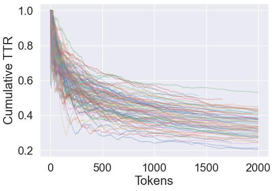

Show code

def MTLD_forward(words, threshold):
    factor = 0
    segment = []
    i = 0
    while i < len(words):
        segment.append(words[i])
        segTTR = TTR(segment)
        if segTTR <= threshold:
            segment = []
            factor += 1
        i += 1
    if len(segment) > 0:
        factor += (1.0 - segTTR) / (1.0 - threshold)
    factor = max(1.0, factor)
    mtld = len(words) / factor
    return mtld


def MTLD(words, threshold=0.720):
    if len(words) == 0:
        return 0.0
    forward = MTLD_forward(words, threshold)
    reverse = MTLD_forward(words[::-1], threshold)
    return 0.5 * (forward + reverse)

vocd-D

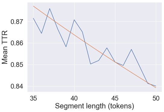
The vocd-D method devised by Malvern et al. (2004) computes the mean TTR across 100 samples of lengths 35, 36, … 49, 50. A function is fit to the resulting TTR vs. sample size data and the extracted best fit parameter \(D\) is the lexical diversity index. Since this is a sampling-based method, the routine is done three times and the average of the \(D\) values is output. I did not have access to Malvern et al. (2004) but did find the relevant function to fit from a publicly viewable implementation that is cited on a Text Inspector page.

\[f_{vocd}(N_s) = \frac{D}{N_s} \left( \sqrt{1 + 2 \frac{N_s}{D}} - 1 \right) \label{vocd-D}\tag{1}\]

where \(N_s\) is the sample size. The higher the value of \(D\), the more diverse the text.

HD-D

McCarthy and Jarvis (2007) showed that vocd-D was merely approximating a result that could directly be computed from the hypergeometric distribution. They developed an alternate implementation HD-D that computes the mean TTR for each sample size by summing the contribution of each type in the text to the overall mean TTR. The contribution of a type \(t\) for a given sample size \(N_s\) is equal to the product of that type’s TTR contribution (\(1/N_s\)) and the probability of finding at least one instance of type \(t\) in any sample. This probability is one minus the probability of finding exactly zero instances of \(t\) in any sample, which can be computed by the hypergeometric distribution \(P_t(k_t=0, N, n_t, N_s)\), where \(k_t\) is the number of instances of type \(t\), \(N\) is still the number of tokens in the text, and \(n_t\) is the number of occurences of \(t\) in the full text (the order of arguments here is chosen to match the input of scipy.stats.hypergeom rather than the example in McCarthy and Jarvis (2007)). Thus, in summary, the goal is to compute

\[f_{HD}(N_s) = \frac{1}{N_s} \sum_{t=1}^{V} 1 - P_t(0, N, n_t, N_s) \label{HD-D}\tag{2}\]

and either equate this to the Eq. \ref{vocd-D} above and solve for \(D\):

\[D(N_s) = -\frac{\left[f_{HD}(N_s)\right]^2}{2\left[f_{HD}(N_s)-1\right]}\]

where \(x\) is the output of Eq. \ref{HD-D}. The average across all sample sizes gives the value of \(D\) for the HD-D method. Alternatively one can instead fit Eq. \ref{vocd-D} to the output of Eq. \ref{HD-D} to determine \(D\).

vocd-D or HD-D?

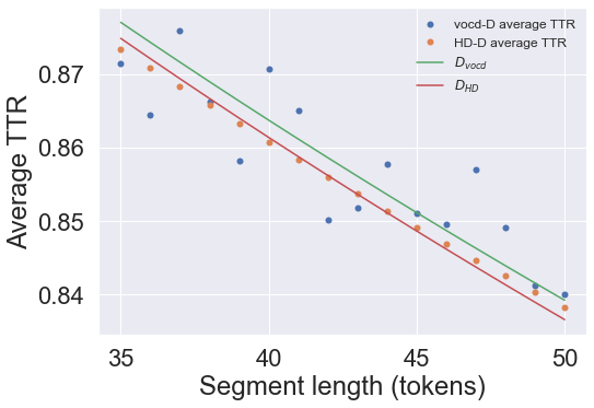
Although vocd-D merely approximates the result of HD-D, the latter is much slower, taking several seconds to produce D for a single artist’s lyrics. The approximate method is still fairly accurate (within <1% away from the HD-D result in the example case) with just three trials, so it is the preferred method used in the rest of the notebook.

Show code

# Example of one vocd-D trial for a single artist

words = df_bands.loc['A Canorous Quintet'].words
num_segs = 100
seglen_range = range(35, 51)
ttrs = np.zeros((len(seglen_range), num_segs))
for i, seglen in enumerate(seglen_range):
    for j in range(num_segs):
        sample = random.sample(words, seglen)
        ttrs[i, j] = TTR(sample)
avg_ttrs_vocdD = ttrs.mean(1)
curve = lambda x, D: (D / x) * (np.sqrt(1 + 2 * (x / D)) - 1)
(D_vocdD,), _ = curve_fit(curve, seglen_range, avg_ttrs_vocdD)
print(D_vocdD)

plt.plot(seglen_range, avg_ttrs_vocdD)
plt.plot(seglen_range, curve(seglen_range, D_vocdD))
plt.xlabel('Segment length (tokens)')
plt.ylabel('Mean TTR')
plt.show()

109.51382921462954

Show code

# vocd-D implementation and example D values

def vocdD_curve(x, D):
    return (D / x) * (np.sqrt(1 + 2 * (x / D)) - 1)

def vocdD(words, num_trials=3, num_segs=100, min_seg=35, max_seg=50):
    if max_seg > len(words):
        return np.nan
    D_trials = []
    seglen_range = range(min_seg, max_seg + 1)
    for _ in range(num_trials):
        ttrs = np.zeros((len(seglen_range), num_segs))
        for i, seglen in enumerate(seglen_range):
            for j in range(num_segs):
                sample = random.sample(words, seglen)
                ttrs[i, j] = TTR(sample)
        avg_ttrs = ttrs.mean(1)
        (D_trial,), _ = curve_fit(vocdD_curve, seglen_range, avg_ttrs)
        D_trials.append(D_trial)
    return np.mean(D_trials)

print(vocdD(df_bands.loc['A Canorous Quintet'].words))
print(vocdD(df_bands.loc['Bal-Sagoth'].words))
print(vocdD(df_bands.loc['Dalriada'].words))

105.70245659158117
100.39975160360206
292.8665221852202

Show code

# Example of HD-D for a single artist and comparison to vocd-D

N = len(words)
types = {t: words.count(t) for t in set(words)}
seglen_range_HDD = range(35, 51)
avg_ttrs_HDD = np.zeros(len(seglen_range_HDD))
D_HDDs = np.zeros(len(seglen_range_HDD))
for s, N_s in enumerate(seglen_range_HDD):
    avg_ttr = 0
    for t, n_t in types.items():
        P_t = hypergeom(N, n_t, N_s).pmf(0)
        avg_ttr += (1 - P_t) / float(N_s)
    avg_ttrs_HDD[s] = avg_ttr
    D_HDDs[s] = -N_s * avg_ttr ** 2 / (2 * (avg_ttr - 1))
D_HDD1 = D_HDDs.mean()
print(D_HDD1)
(D_HDD2,), _ = curve_fit(vocdD_curve, seglen_range, avg_ttrs_HDD)
print(D_HDD2)

plt.plot(seglen_range, avg_ttrs_vocdD, 'o', label='vocd-D average TTR')
plt.plot(seglen_range, avg_ttrs_HDD, 'o', label='HD-D average TTR')
plt.plot(seglen_range, vocdD_curve(seglen_range, D_vocdD), label='$$D_{vocd}$$')
plt.plot(seglen_range, vocdD_curve(seglen_range, np.mean([D_HDD1, D_HDD2])), label='$$D_{HD}$$')
plt.xlabel('Segment length (tokens)')
plt.ylabel('Average TTR')
plt.legend(fontsize=12)
plt.show()

107.01527500420116
107.1183411481678

Show code

def get_lexical_diversity(data):
    N = data.words.apply(len)
    V = data.words.apply(lambda x: len(set(x)))
    data['N'] = N
    data['V'] = V
    data['TTR'] = V / N
    data['rootTTR'] = V / np.sqrt(N)
    data['logTTR'] = np.log(V) / np.log(N)
    data['mtld'] = data.words.apply(MTLD, threshold=0.5)
    data['logmtld'] = np.log(data['mtld'])
    data['vocdd'] = data.words.apply(vocdD, num_segs=10)
    return data[data.N > 0]


df_bands = get_lexical_diversity(df_bands)
df_songs = get_lexical_diversity(df_songs)

Histograms

Show code

def plot_histograms(data):
    fig, axes = plt.subplots(3, 2, figsize=(16, 18))
    fig.suptitle("Lexical diversity of heavy metal artists", fontsize=30)
    axes = axes.flatten()

    ax = axes[0]
    logNmin, logNmax = np.log10(data.N.min()), np.log10(data.N.max())
    logbins = np.logspace(logNmin, logNmax, 20)
    data.N.hist(bins=logbins, edgecolor='k', ax=ax)
    ax.set_xscale('log')
    ax.set_title("Vocabulary sizes")
    ax.set_xlabel("N (tokens)")
    for axis in [ax.xaxis, ax.yaxis]:
        axis.set_major_formatter(ScalarFormatter())

    ax = axes[1]
    data.TTR.hist(bins=20, edgecolor='k', ax=ax)
    ax.set_title("Type-token ratio")
    ax.set_xlabel("$$\mathrm{LD_{TTR} = V/N}$$")

    ax = axes[2]
    data.rootTTR.hist(bins=20, edgecolor='k', ax=ax)
    ax.set_title("Root type-token ratio")
    ax.set_xlabel("$$\mathrm{LD_{rootTTR}} = \sqrt{V/N}$$")

    ax = axes[3]
    data.logTTR.hist(bins=30, edgecolor='k', ax=ax)
    ax.set_title("Logarithmic type-token ratio")
    ax.set_xlabel("$$\mathrm{LD_{logTTR}} = \log V / \log N$$")

    ax = axes[4]
    data.logmtld[data.logmtld > -np.inf].hist(bins=30, edgecolor='k', ax=ax)
    ax.set_title("Measure of Textual Lexical Diversity")
    ax.set_xlabel("$$\log(\mathrm{MTLD})$$")

    ax = axes[5]
    data.vocdd[~data.vocdd.isnull()].hist(bins=30, edgecolor='k', ax=ax)
    ax.set_title("vocd-D")
    ax.set_xlabel("$$D_{\mathrm{fit}}$$")

    for ax in axes:
        ax.set_ylabel("Artists", rotation=0, labelpad=40)
        ax.grid(None)
        ax.grid(axis='y', color='k')

    fig.tight_layout(rect=[0, 0, 1, 0.95])
    return

plot_histograms(df_bands)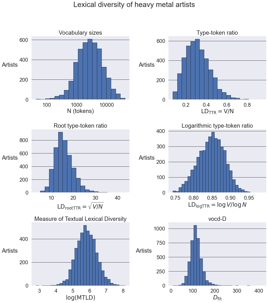

Songs ranked by lexical diversity

Several of the highest MTLD scores come from Bal-Sagoth songs. These are inflated as discussed in Part 1: Bal-Sagoth’s lyrics consist of entire chapters of prose that are not actually sung in the songs themselves. The top band, Ásmegin, also has their MTLD inflated, in their case due to the fact that both Norwegian and English lyrics are posted to DarkLyrics for each song. Bilingual lyrics and unsung commentary likewise inflate the lyrics of Cripple Bastards’ songs, and likewise that of Dalriada’s Zách Klára. These exceptions aside, the highest MTLD song is Divina Enema’s avant-garde metal track Gargoyles Ye Rose Aloft.

There’s a pretty big difference between the MTLD and vocd-D charts, with no bands shared in common among the top-ten of each metric. MTLD seems to weigh longer lyrics more heavily, while vocd-D almost seems to be reflecting TTR, but at least not with the bias towards extremely short (\(N<10\)) songs.

The bottom of the chart is mostly populated by very short, usually one-word, songs. Of songs with at least ten words, the honor of least lyrically diverse song goes to none other than the magnificent “Thunderhorse” by Dethklok, which consists of the words “ride”, “thunder”, “horse”, “revenge”, and of course “thunderhorse”, uttered a total of 33 times altogether. At such low word counts, vocd-D often can’t yield a score, hence the missing values.

Highest MTLD

Show code

song_cols = list(df_songs.columns)
song_cols_show = list(df_songs.columns[:song_cols.index('song') + 1]) + list(df_songs.columns[song_cols.index('N'):])

pd.options.display.float_format = '{:,.2f}'.format

df_songs.sort_values('mtld', ascending=False).reset_index(drop=True).shift(1).loc[1:10, song_cols_show].convert_dtypes()

	band	genre	song	N	V	TTR	rootTTR	logTTR	mtld	logmtld	vocdd
1	Ásmegin	Viking/Folk Metal	Generalen og Troldharen	1029	613	0.60	19.11	0.93	1,029.00	6.94	216.17
2	Bal-Sagoth	Symphonic/Epic Black Metal	The Obsidian Crown Unbound	2391	993	0.42	20.31	0.89	914.29	6.82	81.36
3	Cripple Bastards	Noisecore (early); Grindcore (later)	Splendore e tenebra	865	472	0.55	16.05	0.91	865.00	6.76	161.77
4	Bal-Sagoth	Symphonic/Epic Black Metal	Six Score and Ten Oblations to a Malefic Avatar	840	453	0.54	15.63	0.91	840.00	6.73	130.15
5	Cripple Bastards	Noisecore (early); Grindcore (later)	La repulsione negli occhi	835	469	0.56	16.23	0.91	835.00	6.73	206.22
6	Cripple Bastards	Noisecore (early); Grindcore (later)	When Immunities Fall	816	492	0.60	17.22	0.92	816.00	6.70	210.61
7	Dalriada	Folk Metal	Zách Klára	799	467	0.58	16.52	0.92	799.00	6.68	246.61
8	Divina Enema	Avant-garde Metal	Gargoyles Ye Rose Aloft	842	419	0.50	14.44	0.90	789.38	6.67	143.85
9	Ulver	Black/Folk Metal (early); Ambient/Avant-garde/...	Stone Angels	769	418	0.54	15.07	0.91	769.00	6.65	162.67
10	Bal-Sagoth	Symphonic/Epic Black Metal	Summoning the Guardians of the Astral Gate	759	404	0.53	14.66	0.90	759.00	6.63	87.29

Highest vocd-D

Show code

df_songs.sort_values('vocdd', ascending=False).reset_index(drop=True).shift(1).loc[1:10, song_cols_show].convert_dtypes()

	band	genre	song	N	V	TTR	rootTTR	logTTR	mtld	logmtld	vocdd
1	Hail of Bullets	Death Metal	DAK	54	54	1.00	7.35	1.00	54	3.99	787,177.13
2	Cadaveria	Black/Gothic Metal	Exercise1	119	119	1.00	10.91	1.00	119	4.78	787,177.13
3	Cenotaph	Brutal Death Metal	Voluptuously Minced	67	66	0.99	8.06	1.00	67	4.20	2,095.87
4	Yearning	Atmospheric Doom Metal	Elegy of Blood	56	55	0.98	7.35	1.00	56	4.03	1,576.67
5	Sempiternal Deathreign	Death/Doom Metal	Devastating Empire Towards Humanity	75	73	0.97	8.43	0.99	75	4.32	1,455.21
6	Incantation	Death Metal	Invoked Infinity	53	52	0.98	7.14	1.00	53	3.97	1,432.34
7	Houwitser	Brutal Death Metal	Vile Amputation	53	52	0.98	7.14	1.00	53	3.97	1,379.03
8	Kill the Client	Grindcore	As Roaches	52	51	0.98	7.07	1.00	52	3.95	1,378.93
9	Incantation	Death Metal	Ancients Arise	73	71	0.97	8.31	0.99	73	4.29	1,131.15
10	Venom	NWOBHM/Black/Speed Metal	All There Is Fear	78	75	0.96	8.49	0.99	78	4.36	1,078.96

Lowest MTLD

Show code

df_songs[df_songs.N > 10].sort_values('mtld', ascending=True).reset_index(drop=True).shift(1).loc[1:10, song_cols_show].convert_dtypes()

	band	genre	song	N	V	TTR	rootTTR	logTTR	mtld	logmtld	vocdd
1	Dethklok	Melodic Death Metal	Thunderhorse	33	5	0.15	0.87	0.46	2.95	1.08	<NA>
2	Putrid Pile	Brutal Death Metal	Toxic Shock Therapy	18	3	0.17	0.71	0.38	3.30	1.19	<NA>
3	Axxis	Melodic Heavy/Power Metal	Journey to Utopia	15	2	0.13	0.52	0.26	3.75	1.32	<NA>
4	Katatonia	Doom/Death Metal (early); Gothic/Alternative/P...	Dancing December	12	2	0.17	0.58	0.28	4.00	1.39	<NA>
5	Floodgate	Doom/Stoner Metal	Feel You Burn	56	2	0.04	0.27	0.17	4.00	1.39	0.05
6	Lost Society	Thrash Metal (early); Groove Metal/Metalcore (...	Fatal Anoxia	15	2	0.13	0.52	0.26	4.09	1.41	<NA>
7	M.O.D.	Thrash Metal/Hardcore/Crossover	Bubble Butt	25	5	0.20	1.00	0.50	4.17	1.43	<NA>
8	Dawnbringer	Heavy Metal with Black Metal influences	Scream and Run	51	3	0.06	0.42	0.28	5.44	1.69	0.12
9	Fleshless	Death Metal/Grindcore (early); Melodic/Brutal ...	Evil Odium	11	3	0.27	0.90	0.46	5.81	1.76	<NA>
10	Bloodsoaked	Brutal Technical Death Metal	Devastation Death	12	4	0.33	1.15	0.56	6.00	1.79	<NA>

Lowest vocd-D

Show code

df_songs.sort_values('vocdd', ascending=True).reset_index(drop=True).shift(1).loc[1:10, song_cols_show].convert_dtypes()

	band	genre	song	N	V	TTR	rootTTR	logTTR	mtld	logmtld	vocdd
1	Floodgate	Doom/Stoner Metal	Feel You Burn	56	2	0.04	0.27	0.17	4.00	1.39	0.05
2	Dawnbringer	Heavy Metal with Black Metal influences	Scream and Run	51	3	0.06	0.42	0.28	5.44	1.69	0.12
3	Type O Negative	Gothic/Doom Metal	Set Me on Fire	72	7	0.10	0.82	0.46	9.14	2.21	0.70
4	Hanzel und Gretyl	Industrial Rock (early); Industrial/Groove Met...	Watch TV Do Nothing	54	10	0.19	1.36	0.58	9.90	2.29	1.15
5	Nuit Noire	Black Metal (early); Punk/Black Metal (later)	I Am a Fairy	150	16	0.11	1.31	0.55	10.14	2.32	1.15
6	Mortiis	Darkwave/Dungeon Synth, Electronic/Industrial ...	Thieving Bastards	56	9	0.16	1.20	0.55	9.33	2.23	1.23
7	Vendetta	Thrash Metal	Love Song	55	10	0.18	1.35	0.57	18.52	2.92	1.47
8	Devin Townsend	Progressive Metal, Ambient	Unity	77	12	0.16	1.37	0.57	8.70	2.16	1.55
9	Hanzel und Gretyl	Industrial Rock (early); Industrial/Groove Met...	Hallo Berlin	76	10	0.13	1.15	0.53	13.24	2.58	1.55
10	The Great Kat	Speed/Thrash Metal, Shred	Kill the Mothers	199	22	0.11	1.56	0.58	7.12	1.96	1.55

Bands ranked by lexical diversity

Highest MTLD

Show code

band_cols = list(df_bands.columns)
band_cols_show = ['band', 'genre'] + band_cols[band_cols.index('N'):]

df_bands.sort_values('mtld', ascending=False).reset_index(drop=False).shift(1).loc[1:10, band_cols_show].convert_dtypes()

	band	genre	N	V	TTR	rootTTR	logTTR	mtld	logmtld	vocdd
1	Hail of Bullets	Death Metal	3383	1804	0.53	31.02	0.92	3,383.00	8.13	206.33
2	Demolition Hammer	Thrash Metal (early); Groove Metal (later)	2845	1665	0.59	31.22	0.93	2,845.00	7.95	363.40
3	Malignancy	Brutal Technical Death Metal	6857	2094	0.31	25.29	0.87	2,504.79	7.83	191.29
4	Abnormality	Technical/Brutal Death Metal	2443	1235	0.51	24.99	0.91	2,443.00	7.80	155.92
5	Botanist	Experimental Post-Black Metal	2367	1342	0.57	27.58	0.93	2,367.00	7.77	266.92
6	Moonsorrow	Folk/Pagan/Black Metal	7973	3177	0.40	35.58	0.90	2,344.84	7.76	249.43
7	Thought Industry	Progressive Thrash Metal (early); Alternative ...	2235	1245	0.56	26.33	0.92	2,235.00	7.71	305.54
8	Scrambled Defuncts	Brutal Technical Death Metal	2121	1097	0.52	23.82	0.91	2,121.00	7.66	166.62
9	Brutality	Death Metal	3535	1663	0.47	27.97	0.91	2,106.26	7.65	192.63
10	Metsatöll	Folk Metal	3340	1652	0.49	28.58	0.91	2,044.72	7.62	254.57

Highest vocd-D

Show code

df_bands.sort_values('vocdd', ascending=False).reset_index(drop=False).shift(1).loc[1:10, band_cols_show].convert_dtypes()

	band	genre	N	V	TTR	rootTTR	logTTR	mtld	logmtld	vocdd
1	Krieg	Black Metal	54	51	0.94	6.94	0.99	54.00	3.99	414.42
2	Nortt	Black/Funeral Doom Metal	105	94	0.90	9.17	0.98	105.00	4.65	378.53
3	Demolition Hammer	Thrash Metal (early); Groove Metal (later)	2845	1665	0.59	31.22	0.93	2,845.00	7.95	363.40
4	Four Question Marks	Death Metal, Groove Metal	901	555	0.62	18.49	0.93	901.00	6.80	358.75
5	Virulence	Death Metal/Grindcore with Jazz influences	719	518	0.72	19.32	0.95	719.00	6.58	353.99
6	Terravore	Thrash Metal	1364	869	0.64	23.53	0.94	1,364.00	7.22	308.57
7	Thought Industry	Progressive Thrash Metal (early); Alternative ...	2235	1245	0.56	26.33	0.92	2,235.00	7.71	305.54
8	Dalriada	Folk Metal	5458	2215	0.41	29.98	0.90	1,034.99	6.94	297.45
9	Ásmegin	Viking/Folk Metal	5626	2276	0.40	30.34	0.90	1,337.58	7.20	271.11
10	Botanist	Experimental Post-Black Metal	2367	1342	0.57	27.58	0.93	2,367.00	7.77	266.92

Lowest MTLD

Show code

df_bands.sort_values('mtld', ascending=True).reset_index(drop=False).shift(1).loc[1:10, band_cols_show].convert_dtypes()

	band	genre	N	V	TTR	rootTTR	logTTR	mtld	logmtld	vocdd
1	God Seed	Black Metal	51	22	0.43	3.08	0.79	16.26	2.79	8.88
2	The Great Kat	Speed/Thrash Metal, Shred	2233	509	0.23	10.77	0.81	26.85	3.29	75.45
3	Obús	Heavy Metal/Hard Rock	395	115	0.29	5.79	0.79	31.73	3.46	17.15
4	Dolorian	Black/Doom Metal, Ritual Ambient	1583	397	0.25	9.98	0.81	35.49	3.57	87.97
5	Beyond Black Void	Drone/Funeral Doom Metal	43	34	0.79	5.18	0.94	43.00	3.76	<NA>
6	Steak Number Eight	Atmospheric Sludge/Post-Metal	712	181	0.25	6.78	0.79	46.31	3.84	56.18
7	Svart	Black Metal	47	31	0.66	4.52	0.89	47.00	3.85	<NA>
8	Unida	Stoner Metal	1118	247	0.22	7.39	0.78	49.85	3.91	57.99
9	Krieg	Black Metal	54	51	0.94	6.94	0.99	54.00	3.99	414.42
10	Nuit Noire	Black Metal (early); Punk/Black Metal (later)	963	310	0.32	9.99	0.84	55.39	4.01	52.26

Lowest vocd-D

Show code

df_bands.sort_values('vocdd', ascending=True).reset_index(drop=False).shift(1).loc[1:10, band_cols_show].convert_dtypes()

	band	genre	N	V	TTR	rootTTR	logTTR	mtld	logmtld	vocdd
1	God Seed	Black Metal	51	22	0.43	3.08	0.79	16.26	2.79	8.88
2	Obús	Heavy Metal/Hard Rock	395	115	0.29	5.79	0.79	31.73	3.46	17.15
3	Hämatom	Groove Metal	189	64	0.34	4.66	0.79	60.73	4.11	18.19
4	Saratoga	Power/Heavy Metal	113	56	0.50	5.27	0.85	88.43	4.48	23.72
5	Mystic Forest	Melodic Black Metal	207	88	0.43	6.12	0.84	100.23	4.61	34.62
6	Gris	Black Metal	122	59	0.48	5.34	0.85	122.00	4.80	36.22
7	Bucovina	Black/Folk Metal	238	103	0.43	6.68	0.85	110.66	4.71	37.48
8	EgoNoir	Black Metal	58	40	0.69	5.25	0.91	58.00	4.06	41.01
9	Shadowbreed	Death Metal	306	100	0.33	5.72	0.80	100.38	4.61	42.39
10	Krigere Wolf	Black/Death Metal	830	345	0.42	11.98	0.87	309.29	5.73	43.43

Genres ranked by lexical diversity

Show code

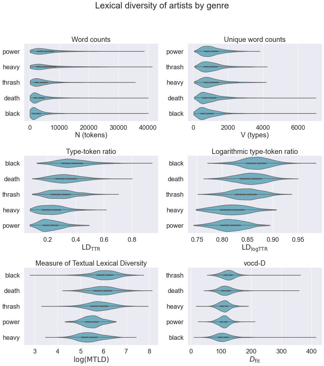
def plot_violinplots(data, figsize=(16, 18)):

    def violinplot(col, ax):
        violindata = []
        labels = data.columns[1:list(data.columns).index('lyrics')]
        for label in labels:
            values = data[data[label] == 1][col]
            values = values[(values > -np.inf) & (values < np.inf)]
            violindata.append((label, values))
        violindata.sort(key=lambda x: -x[1].median())
        plot_labels, plot_data = zip(*violindata)
        sns.violinplot(data=plot_data, cut=0, orient='h', ax=ax, color='c')
        ax.set_yticklabels(plot_labels)
        return

    fig, axes = plt.subplots(3, 2, figsize=figsize)
    fig.suptitle("Lexical diversity of artists by genre", fontsize=30)
    axes = axes.flatten()

    ax = axes[0]
    violinplot('N', ax)
    ax.set_title("Word counts")
    ax.set_xlabel("N (tokens)")

    ax = axes[1]
    violinplot('V', ax)
    ax.set_title("Unique word counts")
    ax.set_xlabel("V (types)")

    ax = axes[2]
    violinplot('TTR', ax)
    ax.set_title("Type-token ratio")
    ax.set_xlabel(r"$$\mathrm{LD_{TTR}}$$")

    ax = axes[3]
    violinplot('logTTR', ax)
    ax.set_title("Logarithmic type-token ratio")
    ax.set_xlabel(r"$$\mathrm{LD_{logTTR}}$$")

    ax = axes[4]
    violinplot('logmtld', ax)
    ax.set_title("Measure of Textual Lexical Diversity")
    ax.set_xlabel("$$\log(\mathrm{MTLD})$$")

    ax = axes[5]
    violinplot('vocdd', ax)
    ax.set_title("vocd-D")
    ax.set_xlabel("$$D_{\mathrm{fit}}$$")

    fig.tight_layout(rect=[0, 0, 1, 0.95])
    return

plot_violinplots(df_bands, figsize=(16, 18))