Reviews of Heavy Metal Albums - Part 2: Review Score Prediction
This article is a part of my heavy metal lyrics project. If you’re interested in seeing the code, check out the original notebook.
Summary
Things we’ll do:
- Convert album review text into machine-learning-ready token sequences
- Use a word embedding from GloVe to convert tokens into word vectors
- Train a convolutional neural network to predict scores of album reviews.
- Visualize neural network training/performance and compare results to that of random guessing.
Table of Contents
Module imports
import re
import pandas as pd
import numpy as np
import matplotlib.pyplot as plt
import seaborn as sns
sns.set(font_scale=2)
from tensorflow import keras
from keras import layers
from keras.models import Sequential
from sklearn.model_selection import train_test_split
Dataset
df = pd.read_csv('E:/Projects/metallyrics/data/new/reviews.csv')
df['review_title'], df['review_score'] = df['review_title'].str.extract('(.*) - (\d+)%').values.T
df['review_score'] = df['review_score'].astype(int)
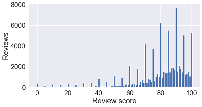
hist = df['review_score'].value_counts().sort_index()
plt.figure(figsize=(10, 5))
plt.bar(hist.index, hist.values, width=1)
plt.xlabel("Review score")
plt.ylabel("Reviews")
plt.show()
Review score prediction using Glove word embeddings
Data preprocessing
X = df['review_content']
y = df['review_score'] / 100
X_train, X_test, y_train, y_test = train_test_split(X, y, test_size=0.2)
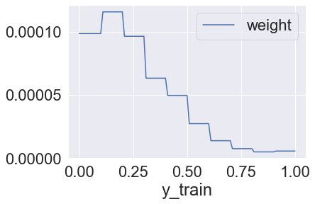
Sample weights
train_hist = y_train.value_counts().sort_index()
intervals = pd.cut(train_hist.index, np.linspace(y.min(), y.max(), 11), include_lowest=True).categories
bin_counts = np.zeros(len(intervals))
for i, interval in enumerate(intervals):
    for j in train_hist.index:
        if j in interval:
            bin_counts[i] += train_hist[j]
sample_bins = np.zeros(len(y_train), dtype=int)
for i, y in enumerate(y_train):
    for j, interval in enumerate(intervals):
        if y in interval:
            sample_bins[i] = j
            break
sample_weights = 1.0 / bin_counts[sample_bins]
sample_weights /= sample_weights.sum()
pd.DataFrame(np.column_stack([y_train, sample_bins, sample_weights]), columns=["y_train", "bin", "weight"]).convert_dtypes().sort_values('y_train').plot('y_train', 'weight')
plt.show()
Convert text to padded sequences of tokens
tokenizer = keras.preprocessing.text.Tokenizer(filters='!"#$%&()*+,-./:;<=>?@[\\]^_`{|}~\t\n\r\'')
tokenizer.fit_on_texts(X_train)
vocab_size = len(tokenizer.index_word) + 1
print(f"vocabulary size: {vocab_size}")
vocabulary size: 256786
def texts_to_padded(texts, maxlen=None):
    sequences = tokenizer.texts_to_sequences(texts)
    padded = keras.preprocessing.sequence.pad_sequences(sequences, padding='post', maxlen=maxlen)
    return padded
padded_train = texts_to_padded(X_train)
padded_test = texts_to_padded(X_test)
pd.DataFrame(np.sum(padded_train > 0, axis=1), columns={"Sequence length"}).describe()
| Sequence length | |
|---|---|
| count | 69160.000000 |
| mean | 601.691281 |
| std | 281.243588 |
| min | 91.000000 |
| 25% | 415.000000 |
| 50% | 549.500000 |
| 75% | 724.000000 |
| max | 5769.000000 |
print(padded_train.shape, y_train.shape, padded_test.shape, y_test.shape)
(69160, 5769) (69160,) (17290, 6849) (17290,)
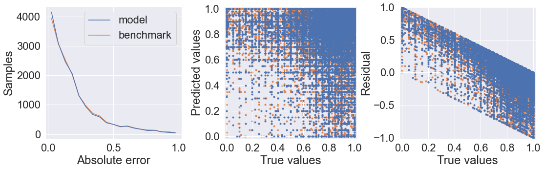
Benchmark model
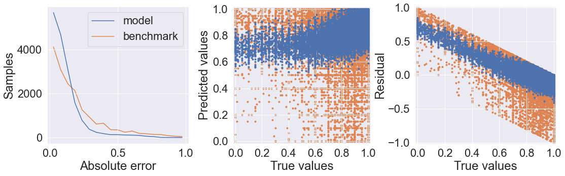
This benchmark model “predicts” scores by sampling from the distribution of scores in the training data, so it represents the outcome of informed random guessing.
train_pdf = y_train.value_counts().sort_index()
train_cdf = train_pdf.cumsum() / train_pdf.sum()


def benchmark_predict(n_samples):
    r = np.random.rand(n_samples)
    pred_idx = np.argmax((train_cdf.values[:, None] - r) > 0, axis=0)
    pred = train_cdf.index[pred_idx]
    return pred

def evaluate_prediction(pred, true, benchmark=False):
    fig, (ax1, ax2, ax3) = plt.subplots(1, 3, figsize=(18, 5))
    fig.subplots_adjust(wspace=0.3)
    bins = np.linspace(0, 1, 20)
    hist, bins = np.histogram(np.abs(pred - true), bins=bins)
    bin_centers = bins[:-1] + np.diff(bins)[0] / 2
    ax1.plot(bin_centers, hist, label="model", zorder=1)
    ax2.plot(true, pred, '.', zorder=1)
    ax3.plot(true, pred - true, '.', zorder=1)
    if benchmark:
        y_bench = benchmark_predict(len(true))
        hist_bm, _ = np.histogram(np.abs(y_bench - true), bins=bins)
        ax1.plot(bin_centers, hist_bm, label="benchmark", zorder=0)
        ax2.plot(true, y_bench, '.', zorder=0)
        ax3.plot(true, y_bench - true, '.', zorder=0)
    ax1.set_xlabel("Absolute error")
    ax1.set_ylabel("Samples")
    ax1.legend()
    ax2.set_xlabel("True values")
    ax2.set_ylabel("Predicted values")
    ax2.set_xlim(-0.02, 1.02)
    ax2.set_ylim(-0.02, 1.02)
    ax2.set_xticks(np.linspace(0, 1, 6))
    ax2.set_yticks(np.linspace(0, 1, 6))
    ax2.set_aspect('equal')
    ax3.set_xlabel("True values")
    ax3.set_ylabel("Residual")
    ax3.set_xlim(-0.02, 1.02)
    ax3.set_ylim(-1.02, 1.02)
    ax3.set_xticks(np.linspace(0, 1, 6))
    ax3.set_yticks(np.linspace(-1, 1, 5))
    plt.show()

evaluate_prediction(benchmark_predict(len(y_test)), y_test, benchmark=True)
Load word vectors and create an embedding layer
Adapted from a Keras tutorial.
Here I create a word embedding layer in order to convert each token in each sequence into a word vector. I use a pre-trained word embedding, the 6-billion-token, 100-dimensional Wikipedia+Gigaword 5 word embedding from GloVe. This transforms each token into a 100-dimensional vector whose location in the word vector space represents its association to nearby word vectors. The full dataset will therefore be represented as a matrix of shape (number of samples, sequence length, 100).
path_to_glove_file = "E:/Projects/metallyrics/data/glove.6B.100d.txt"

embedding_vectors = {}
with open(path_to_glove_file, encoding="utf8") as f:
    for line in f:
        word, coefs = line.split(maxsplit=1)
        coefs = np.fromstring(coefs, "f", sep=" ")
        embedding_vectors[word] = coefs
print(len(embedding_vectors))
print(len(list(embedding_vectors.values())[0]))
400001
100
embedding_dim = len(list(embedding_vectors.values())[0])
hits = 0
misses = 0

# Prepare embedding matrix
embedding_matrix = np.zeros((vocab_size, embedding_dim))
for word, i in tokenizer.word_index.items():
    embedding_vector = embedding_vectors.get(word)
    if embedding_vector is not None:
        if len(embedding_vector) > 0:
            # Words not found in embedding index will be all-zeros.
            # This includes the representation for "padding" and "OOV"
            embedding_matrix[i] = embedding_vector
            hits += 1
            continue
    misses += 1
print("Converted %d words (%d misses)" % (hits, misses))
Converted 84032 words (172753 misses)
As an example, we can see look at the 10 nearest words to “fire”, based on cosine distance.
vector = embedding_vectors['fire']
cos_dist = np.dot(embedding_matrix, vector) / (np.linalg.norm(embedding_matrix, axis=1) * np.linalg.norm(vector))
cos_dist = np.nan_to_num(cos_dist, 0)
print([tokenizer.index_word.get(i, 0) for i in cos_dist.argsort()][:-11:-1])
['fire', 'fires', 'fired', 'firing', 'attack', 'explosion', 'blast', 'blaze', 'police', 'ground']


C:\Users\philn\AppData\Local\Temp\ipykernel_11568\952163309.py:2: RuntimeWarning: invalid value encountered in true_divide
  cos_dist = np.dot(embedding_matrix, vector) / (np.linalg.norm(embedding_matrix, axis=1) * np.linalg.norm(vector))
embedding_layer = layers.Embedding(
    vocab_size,
    embedding_dim,
    embeddings_initializer=keras.initializers.Constant(embedding_matrix),
    trainable=False,
)
Convolutional Neural Network
After a little manual hyperparameter tuning (tweaking the number of filters, dense layer size, learning rate, and regularization methods), I found that this model was unable to learn at all using mean squared error (MSE) for the loss function. Mean absolute error (MAE) worked instantly when implemented. This is probably because MSE does well at punishing outliers, but there the review score range is bounded, so there are no huge outliers in the data.
I also tested it with and without sample weighting since the test samples are heavily distributed in favor of high-scoring reviews. I found that with sample weighting, the model was less likely to overestimate the scores of negative reviews. However, the residual plots show that there is still a decent amount of bias towards overestimating scores, although it does perform much better than the random sampling benchmark.
Any further tuning should probably be done with cross-validation just to robust, but I’m pretty happy with the model as is so I’m leaving it as is.
Also, I tried training a recurrent neural network on the data and it miserably overfit, and tuning took too long because of the very slow training time. Oh well, I’m happy with the ConvNet!
cnn_model = Sequential()
cnn_model.add(embedding_layer)
cnn_model.add(layers.Conv1D(filters=128, kernel_size=5, activation='relu'))
cnn_model.add(layers.BatchNormalization())
cnn_model.add(layers.GlobalMaxPooling1D())
cnn_model.add(layers.Flatten())
cnn_model.add(layers.Dense(64))
cnn_model.add(layers.Dropout(0.2))
cnn_model.add(layers.Dense(1, activation='linear'))
opt = keras.optimizers.Adam(learning_rate=0.001)
cnn_model.compile(optimizer=opt, loss='mean_absolute_error', metrics=['mae'])
print(cnn_model.summary())
Model: "sequential"
_________________________________________________________________
 Layer (type)                Output Shape              Param #
=================================================================
 embedding (Embedding)       (None, None, 100)         25678600

 conv1d (Conv1D)             (None, None, 128)         64128

 batch_normalization (BatchN  (None, None, 128)        512
 ormalization)

 global_max_pooling1d (Globa  (None, 128)              0
 lMaxPooling1D)

 flatten (Flatten)           (None, 128)               0

 dense (Dense)               (None, 64)                8256

 dropout (Dropout)           (None, 64)                0

 dense_1 (Dense)             (None, 1)                 65

=================================================================
Total params: 25,751,561
Trainable params: 72,705
Non-trainable params: 25,678,856
_________________________________________________________________
None
early_stopping = keras.callbacks.EarlyStopping(
    monitor="val_loss",
    min_delta=0,
    patience=10,
    verbose=0,
    mode="auto",
    baseline=None,
    restore_best_weights=True,
)
cnn_history = cnn_model.fit(
    padded_train[::10],
    y_train[::10],
    batch_size=32,
    callbacks=[early_stopping],
    epochs=64,
    sample_weight=sample_weights,
    validation_split=0.2,
    verbose=1
)
Epoch 1/64
173/173 [==============================] - 88s 500ms/step - loss: 5.8694e-05 - mae: 4.1086 - val_loss: 1.4992e-05 - val_mae: 1.0833
Epoch 2/64
173/173 [==============================] - 93s 539ms/step - loss: 2.0165e-05 - mae: 1.3171 - val_loss: 1.2310e-05 - val_mae: 0.8717
Epoch 3/64
173/173 [==============================] - 94s 544ms/step - loss: 1.6722e-05 - mae: 1.1126 - val_loss: 4.7313e-06 - val_mae: 0.3427
Epoch 4/64
173/173 [==============================] - 91s 527ms/step - loss: 8.8949e-06 - mae: 0.6018 - val_loss: 4.9187e-06 - val_mae: 0.3581
Epoch 5/64
173/173 [==============================] - 90s 523ms/step - loss: 8.4884e-06 - mae: 0.5732 - val_loss: 5.2625e-06 - val_mae: 0.3796
Epoch 6/64
173/173 [==============================] - 90s 522ms/step - loss: 5.8895e-06 - mae: 0.3963 - val_loss: 4.2899e-06 - val_mae: 0.2966
Epoch 7/64
173/173 [==============================] - 90s 523ms/step - loss: 5.2813e-06 - mae: 0.3673 - val_loss: 2.7561e-06 - val_mae: 0.1980
Epoch 8/64
173/173 [==============================] - 91s 527ms/step - loss: 4.5470e-06 - mae: 0.3058 - val_loss: 2.5073e-06 - val_mae: 0.1735
Epoch 9/64
173/173 [==============================] - 93s 538ms/step - loss: 4.5829e-06 - mae: 0.3199 - val_loss: 2.7080e-06 - val_mae: 0.1862
Epoch 10/64
173/173 [==============================] - 93s 535ms/step - loss: 3.7249e-06 - mae: 0.2571 - val_loss: 2.5773e-06 - val_mae: 0.1886
Epoch 11/64
173/173 [==============================] - 95s 547ms/step - loss: 2.9985e-06 - mae: 0.2176 - val_loss: 5.2339e-06 - val_mae: 0.3673
Epoch 12/64
173/173 [==============================] - 92s 533ms/step - loss: 2.7771e-06 - mae: 0.1992 - val_loss: 2.0013e-06 - val_mae: 0.1455
Epoch 13/64
173/173 [==============================] - 91s 527ms/step - loss: 2.4225e-06 - mae: 0.1751 - val_loss: 1.9093e-06 - val_mae: 0.1375
Epoch 14/64
173/173 [==============================] - 89s 516ms/step - loss: 2.6043e-06 - mae: 0.1929 - val_loss: 1.8479e-06 - val_mae: 0.1343
Epoch 15/64
173/173 [==============================] - 94s 542ms/step - loss: 2.2208e-06 - mae: 0.1628 - val_loss: 1.8226e-06 - val_mae: 0.1337
Epoch 16/64
173/173 [==============================] - 94s 541ms/step - loss: 2.2433e-06 - mae: 0.1650 - val_loss: 2.0005e-06 - val_mae: 0.1406
Epoch 17/64
173/173 [==============================] - 91s 524ms/step - loss: 2.0114e-06 - mae: 0.1512 - val_loss: 1.8531e-06 - val_mae: 0.1367
Epoch 18/64
173/173 [==============================] - 89s 515ms/step - loss: 1.8816e-06 - mae: 0.1428 - val_loss: 1.8547e-06 - val_mae: 0.1363
Epoch 19/64
173/173 [==============================] - 87s 504ms/step - loss: 2.0128e-06 - mae: 0.1482 - val_loss: 1.9430e-06 - val_mae: 0.1356
Epoch 20/64
173/173 [==============================] - 90s 521ms/step - loss: 1.9774e-06 - mae: 0.1477 - val_loss: 2.0572e-06 - val_mae: 0.1531
Epoch 21/64
173/173 [==============================] - 92s 534ms/step - loss: 1.9899e-06 - mae: 0.1491 - val_loss: 2.3378e-06 - val_mae: 0.1743
Epoch 22/64
173/173 [==============================] - 90s 519ms/step - loss: 1.9357e-06 - mae: 0.1461 - val_loss: 1.7571e-06 - val_mae: 0.1259
Epoch 23/64
173/173 [==============================] - 88s 511ms/step - loss: 1.8833e-06 - mae: 0.1436 - val_loss: 2.2944e-06 - val_mae: 0.1711
Epoch 24/64
173/173 [==============================] - 87s 502ms/step - loss: 1.9607e-06 - mae: 0.1497 - val_loss: 1.7771e-06 - val_mae: 0.1271
Epoch 25/64
173/173 [==============================] - 89s 517ms/step - loss: 1.8041e-06 - mae: 0.1387 - val_loss: 1.7639e-06 - val_mae: 0.1313
Epoch 26/64
173/173 [==============================] - 91s 524ms/step - loss: 1.8704e-06 - mae: 0.1450 - val_loss: 1.8552e-06 - val_mae: 0.1307
Epoch 27/64
173/173 [==============================] - 89s 512ms/step - loss: 1.9005e-06 - mae: 0.1422 - val_loss: 1.7056e-06 - val_mae: 0.1251
Epoch 28/64
173/173 [==============================] - 92s 530ms/step - loss: 1.8466e-06 - mae: 0.1417 - val_loss: 1.8919e-06 - val_mae: 0.1431
Epoch 29/64
173/173 [==============================] - 86s 500ms/step - loss: 1.8246e-06 - mae: 0.1424 - val_loss: 1.7013e-06 - val_mae: 0.1258
Epoch 30/64
173/173 [==============================] - 94s 541ms/step - loss: 1.7767e-06 - mae: 0.1381 - val_loss: 1.7744e-06 - val_mae: 0.1320
Epoch 31/64
173/173 [==============================] - 87s 506ms/step - loss: 1.6082e-06 - mae: 0.1280 - val_loss: 1.8519e-06 - val_mae: 0.1378
Epoch 32/64
173/173 [==============================] - 86s 496ms/step - loss: 1.6742e-06 - mae: 0.1303 - val_loss: 1.7625e-06 - val_mae: 0.1322
Epoch 33/64
173/173 [==============================] - 86s 497ms/step - loss: 1.9646e-06 - mae: 0.1496 - val_loss: 2.2203e-06 - val_mae: 0.1652
Epoch 34/64
173/173 [==============================] - 86s 497ms/step - loss: 1.5505e-06 - mae: 0.1244 - val_loss: 1.6830e-06 - val_mae: 0.1264
Epoch 35/64
173/173 [==============================] - 86s 497ms/step - loss: 1.5855e-06 - mae: 0.1245 - val_loss: 1.7687e-06 - val_mae: 0.1264
Epoch 36/64
173/173 [==============================] - 86s 496ms/step - loss: 1.5515e-06 - mae: 0.1243 - val_loss: 1.6976e-06 - val_mae: 0.1263
Epoch 37/64
173/173 [==============================] - 86s 499ms/step - loss: 1.6443e-06 - mae: 0.1296 - val_loss: 1.6797e-06 - val_mae: 0.1245
Epoch 38/64
173/173 [==============================] - 86s 495ms/step - loss: 1.6285e-06 - mae: 0.1306 - val_loss: 2.0313e-06 - val_mae: 0.1527
Epoch 39/64
173/173 [==============================] - 87s 500ms/step - loss: 1.4781e-06 - mae: 0.1199 - val_loss: 1.6394e-06 - val_mae: 0.1220
Epoch 40/64
173/173 [==============================] - 92s 532ms/step - loss: 1.3962e-06 - mae: 0.1163 - val_loss: 1.6667e-06 - val_mae: 0.1236
Epoch 41/64
173/173 [==============================] - 88s 509ms/step - loss: 1.5575e-06 - mae: 0.1244 - val_loss: 1.7488e-06 - val_mae: 0.1312
Epoch 42/64
173/173 [==============================] - 87s 503ms/step - loss: 1.3551e-06 - mae: 0.1156 - val_loss: 1.7416e-06 - val_mae: 0.1248
Epoch 43/64
173/173 [==============================] - 86s 500ms/step - loss: 1.3960e-06 - mae: 0.1158 - val_loss: 1.6459e-06 - val_mae: 0.1220
Epoch 44/64
173/173 [==============================] - 85s 494ms/step - loss: 1.5601e-06 - mae: 0.1267 - val_loss: 1.6991e-06 - val_mae: 0.1271
Epoch 45/64
173/173 [==============================] - 86s 497ms/step - loss: 1.4660e-06 - mae: 0.1185 - val_loss: 1.6531e-06 - val_mae: 0.1211
Epoch 46/64
173/173 [==============================] - 86s 499ms/step - loss: 1.4638e-06 - mae: 0.1212 - val_loss: 1.6385e-06 - val_mae: 0.1230
Epoch 47/64
173/173 [==============================] - 85s 493ms/step - loss: 1.3944e-06 - mae: 0.1143 - val_loss: 1.8621e-06 - val_mae: 0.1401
Epoch 48/64
173/173 [==============================] - 86s 495ms/step - loss: 1.3340e-06 - mae: 0.1126 - val_loss: 1.8404e-06 - val_mae: 0.1386
Epoch 49/64
173/173 [==============================] - 86s 495ms/step - loss: 1.3858e-06 - mae: 0.1142 - val_loss: 1.6297e-06 - val_mae: 0.1198
Epoch 50/64
173/173 [==============================] - 85s 493ms/step - loss: 1.3097e-06 - mae: 0.1090 - val_loss: 1.6380e-06 - val_mae: 0.1216
Epoch 51/64
173/173 [==============================] - 86s 497ms/step - loss: 1.2865e-06 - mae: 0.1068 - val_loss: 1.8006e-06 - val_mae: 0.1376
Epoch 52/64
173/173 [==============================] - 87s 503ms/step - loss: 1.2819e-06 - mae: 0.1068 - val_loss: 1.6134e-06 - val_mae: 0.1202
Epoch 53/64
173/173 [==============================] - 87s 501ms/step - loss: 1.2717e-06 - mae: 0.1063 - val_loss: 1.6558e-06 - val_mae: 0.1206
Epoch 54/64
173/173 [==============================] - 86s 498ms/step - loss: 1.2228e-06 - mae: 0.1020 - val_loss: 1.6211e-06 - val_mae: 0.1195
Epoch 55/64
173/173 [==============================] - 86s 495ms/step - loss: 1.4324e-06 - mae: 0.1136 - val_loss: 1.6842e-06 - val_mae: 0.1257
Epoch 56/64
173/173 [==============================] - 85s 494ms/step - loss: 1.3262e-06 - mae: 0.1092 - val_loss: 1.6359e-06 - val_mae: 0.1226
Epoch 57/64
173/173 [==============================] - 85s 494ms/step - loss: 1.2505e-06 - mae: 0.1041 - val_loss: 1.6453e-06 - val_mae: 0.1200
Epoch 58/64
173/173 [==============================] - 86s 497ms/step - loss: 1.1534e-06 - mae: 0.0999 - val_loss: 1.7111e-06 - val_mae: 0.1287
Epoch 59/64
173/173 [==============================] - 89s 512ms/step - loss: 1.1892e-06 - mae: 0.1020 - val_loss: 1.6386e-06 - val_mae: 0.1223
Epoch 60/64
173/173 [==============================] - 90s 519ms/step - loss: 1.1914e-06 - mae: 0.1017 - val_loss: 1.7300e-06 - val_mae: 0.1226
Epoch 61/64
173/173 [==============================] - 89s 514ms/step - loss: 1.1220e-06 - mae: 0.0967 - val_loss: 1.6329e-06 - val_mae: 0.1220
Epoch 62/64
173/173 [==============================] - 90s 520ms/step - loss: 1.1181e-06 - mae: 0.0956 - val_loss: 1.6631e-06 - val_mae: 0.1233
Model assessment
train_metrics = cnn_model.evaluate(padded_train, y_train, verbose=0)
test_metrics = cnn_model.evaluate(padded_test, y_test, verbose=0)
train_metrics = {cnn_model.metrics_names[i]: value for i, value in enumerate(train_metrics)}
test_metrics = {cnn_model.metrics_names[i]: value for i, value in enumerate(test_metrics)}
fig, (ax1, ax2) = plt.subplots(2, 1, figsize=(12, 8))
fig.subplots_adjust(hspace=0.4)
ax1.set_title('Loss')
ax1.plot(cnn_history.history['loss'], label='train')
ax1.plot(cnn_history.history['val_loss'], label='test')
ax1.set_yscale('log')
ax1.legend()
ax2.set_title('Mean Absolute Error')
ax2.plot(cnn_history.history['mae'], label='train')
ax2.plot(cnn_history.history['val_mae'], label='test')
ax2.set_yscale('log')
ax2.legend()
plt.show()
for metric in cnn_model.metrics_names:
    print(f"Train {metric}: {train_metrics[metric]:.2f}")
    print(f"Test  {metric}: {test_metrics[metric]:.2f}")
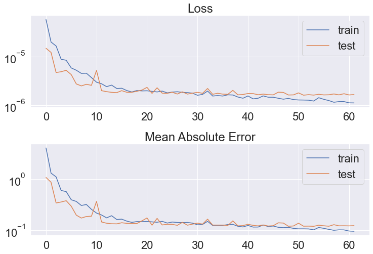
Train loss: 0.12
Test  loss: 0.12
Train mae: 0.12
Test  mae: 0.12
y_pred = cnn_model.predict(padded_test)[:, 0]
y_pred = np.maximum(0, np.minimum(1, y_pred))
evaluate_prediction(y_pred, y_test, benchmark=True)
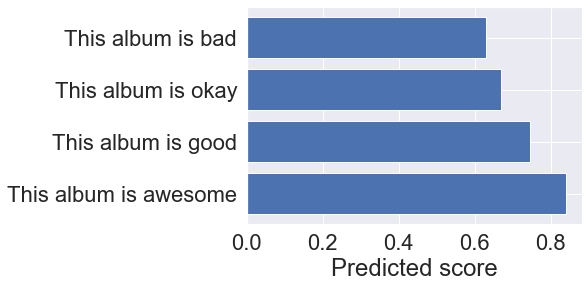
texts = ["This album is bad", "This album is okay", "This album is good", "This album is awesome"]
pred = cnn_model.predict(texts_to_padded(texts, maxlen=padded_train.shape[0]))[:, 0]
plt.barh(range(len(pred)), pred[::-1])
plt.yticks(range(len(pred)), texts[::-1])
plt.xlabel("Predicted score")
plt.show()